Probabilistic Sensitivity Analysis of Misclassification
| Overview | Software |
| Description | Websites |
| Readings | Courses |
Overview
Probabilistic sensitivity analysis is a quantitative method to account for uncertainty in the true values of bias parameters, and to simulate the effects of adjusting for a range of bias parameters. Rather than assuming that one set of bias parameters is most valid, probabilistic methods allow the researcher to specify a plausible distribution of parameters, from which data are sampled to simulate a range of bias-corrected estimates. The methods described herein are illustrated using the context of misclassification, but can also be applied to selection bias, confounding, and other scenarios where bias is likely.
Description
Standard Practices for Bias Analysis
In epidemiologic practice, the practice of quantitative assessments of bias, specifically due to misclassification, is limited. Confidence intervals are used to quantify the uncertainty due to random error around a study’s effect estimate, though systematic errors such as misclassification of study variables should receive equal consideration as sources of bias. In the instances when residual bias in adjusted model estimates is discussed by researchers, it is often qualitative in nature. For example, discussion of misclassification is often dismissed as non-differential and thus biasing estimates toward a null effect, which implies an even larger ‘true’ causal effect. Not only is this assumption often incorrect (e.g., Dosemeci, Wacholder, & Lubin, 1990; Kristensen, 1992), it minimizes a thoughtful appreciation of systematic errors that can lead to violation of modeling assumptions, and cause significant bias in effect estimates and potentially incorrect study inferences.
When misclassification is discussed quantitatively, it is often in the context of sensitivity and specificity of study measures (see table 1 for a review of how these parameters are calculated). That is, when a presumed criterion exists to which measures can be compared. Positing, for example, that an exposure was measured with a sensitivity of 0.9 (i.e., the probability that those who were truly exposed were classified as exposed) and a specificity of 0.8 (i.e., the probability that those who were truly unexposed were classified as unexposed), allows a researcher to back-calculate the ‘true’ exposure and disease values. In this way, independent and dependent non-differential, differential misclassification of any study variable can be examined. However, this method implies that one set of misclassification parameters are the most plausible and valid (Fox, Lash, & Greenland, 2005), leading to a similar overconfidence in adjusted measures.
Table 1. Sensitivity, specificity, positive predictive value, and negative predictive value of observed study variables.
|
|
|
True status |
|
|
|
|
Positive |
Negative |
||
|
As measured |
Positive |
True Positive (TP) |
False Positive (FP) |
TP+FP |
|
Negative |
False Negative (FN) |
True Negative (TN) |
TN+FN |
|
|
|
TP+FN |
FP+TN |
||
Sensitivity = Pr(TP | TP + FN)
Specificity = Pr(TN | TN + FP)
Positive Predictive Value = Pr(TP | TP + FP)
Negative Predictive Value = Pr(TN | TN + FN)
Monte-Carlo Sensitivity Analysis
Methods have been developed to account for uncertainty in the true values of bias parameters, and to simulate the effects of adjusting for a range of sensitivity and specificity values. One such method, Monte Carlo Sensitivity Analysis (MCSA) allows the researcher to specify a plausible distribution of parameters, from which data are probabilistically sampled to simulate a range of bias-corrected estimates.
MCSA implementation
The following is a general description of how an MCSA simulation is implemented:
-
The user must input the observed data, either as a dataset or as a summary 2x2 contingency table. The type of misclassification to be adjusted must also be specified (e.g., exposure or disease).
-
Specify parameter distributions: The parameter distributions should be predetermined by the researcher, based on thoughtful hypotheses, consultations with experts, and reviews of the literature (Greenland & Lash, 2008). If non-differential misclassification is hypothesized, two distributions are specified (i.e., sensitivity and specificity), while if differential misclassification is suspected, four parameters are input (i.e., two sensitivity and specificity parameters, different by exposure or disease status). Each parameter consists of the probability distribution function, which is a simplified shape of the distribution that defines the probability of selecting sensitivity/specificity values. Generally, it is necessary to specify a lower and upper bound in the parameter range, which respectively increase and decrease around either a zone or a point where all probabilities are equally likely to be selected.
-
Specify the number of replications on the simulation. Each replication involves selecting one sensitivity and specificity value from the probability distribution to be used to calculate the positive and negative predictive values (PPV, NPV, respectively). These PPV and NPV values represent the probability that a subject was correctly classified, given their observed exposure and disease status. The number of replications may be increased as the parameter range increases. The PPV and NPV are derived from the following steps:
1. The selected sensitivity and specificity are used to back-calculate the expected exposed/ unexposed cases from the observed data, using the following equations:
A = [a – (1–S0) * N]/[S1–(1–S0)]
B = N–A
Where, S1 = Sensitivity; S0 = Specificity;
N = Total cases
A = expected exposed cases; a = observed exposed cases
B = expected unexposed cases; b = observed unexposed cases
2. From the expected cases, the expected number of true/false positives and negatives are calculated, using the following equations:
T1 = S1 * A
T0 = S0 * B
F1 = (1–S0) * B
F0 = (1–S1) * A
Where, T1 = expected true positives; T0 = expected true negatives
F1 = expected false positives; F0 = expected false negatives
3. From these, the PPV and NPV are calculated, using the following equations:
PPV = T1 / (T1 + F1)
NPV = T0 / (T0 + F0)
IV. Given the PPV and NPV, each replication recreates the entire dataset by completing a Bernoulli trial (Lash & Fink, 2003). For each individual i, a random number X from a uniform distribution [0,1] is chosen.
-
Given i is observed exposed, if X > PPV, then i is reclassified as unexposed.
-
Given i is observed unexposed, if X > NPV, then i is reclassified as exposed.
Because the bias adjustments are made at the level of the individual record, it is possible to include additional covariate adjustments at this point.
V. From these bias-adjusted datasets, an effect estimate is calculated. From the entire set of adjusted estimates a simulation interval is calculated, given the specified alpha level. In addition, to account for random error in the adjusted estimates, the observed standard deviation is multiplied by a random standard normal deviate, which is subtracted from the bias-adjusted point estimate, as shown in the formula below (Greenland, 2005). It is also possible to use bootstrap methods to incorporate random error through resampling the adjusted datasets (Davison & Hinkley, 1997).

Where, zi random deviate from a standard normal distribution
MCSA output includes three sets of estimates: 1) the observed effect estimate and its 95% confidence interval; 2) the median effect estimate and its simulation interval adjusted for only systematic errors, and 3) the effect estimate and its simulation interval adjusted for systematic and random errors. Tools to implement MCSA for many types of bias are available in nearly all major statistical software packages. See appendix 1 for a list of available types of bias analysis by program.
Limitations and general strategy
There are an increasing number of examples of how this type of analysis may be presented in the literature (e.g., Hoefler, Lieb, & Wittchen, 2007; Stonebraker, Farrugia, Gathmann, Orange, & Party, 2014). Specific guidelines for a comprehensive bias analysis are available (Greenland, 1996; Lash et al., 2014) and should replace the current standard which does not take seriously the possibility of systematic bias in study estimates.
There are limitations to MCSA methods. Their valid implementation rests on the assumption that the type and degree of bias is correctly specified. While specifying a distribution of bias parameters implies a much less stringent assumption than using a single set of sensitivity/specificity values, these prior distributions may be contested by reviewers or other researchers in the field. As Greenland (2001, p. 582) noted in his discussion of these methods, “A prior distribution is credible if it has an explicit rationale and is plausible for all concerned parties.” The value of MCSA and similar Bayesian methods (Gustafson, 2003) is in forcing the researcher to specify the prior assumptions underlying the validity of the variables used in their analysis, based on thoughtful hypotheses and previous research on similar topics. At this point, there is no consensus about how best to construct prior distributions (Lash et al., 2014); relying too heavily on prior research or expert opinions may introduce bias into the analysis based on subjective opinions and publication bias. Despite this and other evolving issues, MCSA represents a movement toward a more transparent discussion of the nature of bias and will likely improve the ability of epidemiologists to produce and replicate valid research.
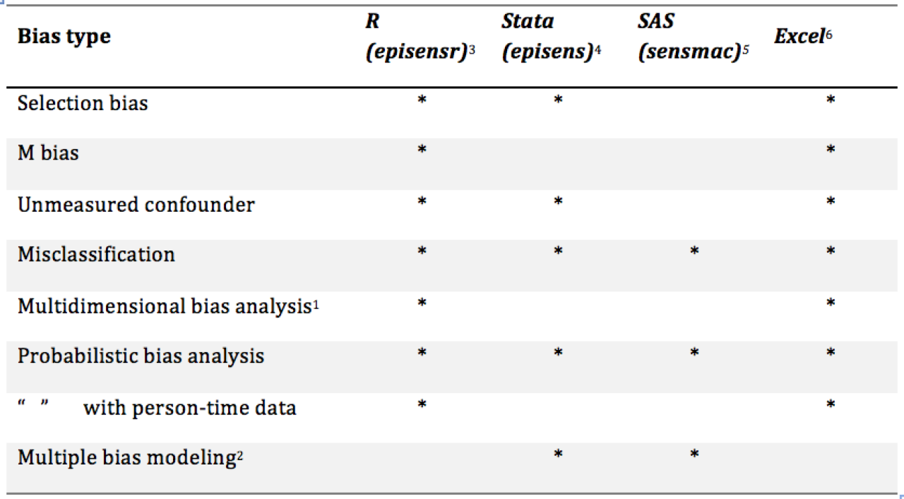
Appendix 1. Available quantitative bias sensitivity analyses in episensr and other statistical software packages (adapted from: Lash, Fox, & Fink, 2011).
1 Refers to analysis where multiple bias parameters are considered for one type of bias.
2 Refers to analysis where multiple types of bias are considered and successively tested.
3 Available at: https://cran.r-project.org/web/packages/episensr/episensr.pdf
4 Available at: www.stata-journal.com/sjpdf.html?articlenum=st0138
5 Available at: https://sites.google.com/site/biasanalysis/sensmac
6 Available at: https://sites.google.com/site/biasanalysis/
References
Briggs, A. H., Weinstein, M. C., Fenwick, E. A., Karnon, J., Sculpher, M. J., & Paltiel, A. D. (2012). Model parameter estimation and uncertainty analysis a report of the ISPOR-SMDM Modeling Good Research Practices Task Force Working Group–6. Medical Decision Making, 32(5), 722-732.
Davison, A. C., & Hinkley, D. V. (1997). Bootstrap methods and their application (Vol. 1): Cambridge university press.
Dosemeci, M., Wacholder, S., & Lubin, J. H. (1990). Does nondifferential misclassification of exposure always bias a true effect toward the null value? American journal of epidemiology, 132(4), 746-748.
Fox, M. P., Lash, T. L., & Greenland, S. (2005). A method to automate probabilistic sensitivity analyses of misclassified binary variables. International Journal of Epidemiology, 34(6), 1370-1376.
Greenland, S. (2005). Multiple‐bias modelling for analysis of observational data. Journal of the Royal Statistical Society: Series A (Statistics in Society), 168(2), 267-306.
Greenland, S., & Lash, T. L. (2008). Bias analysis. In K. J. Rothman, S. Greenland, & T. L. Lash (Eds.), Modern epidemiology (3 ed., pp. 345-380). Philadelphia: Lippincott Williams & Wilkins.
Kristensen, P. (1992). Bias from nondifferential but dependent misclassification of exposure and outcome. Epidemiology, 210-215.
Lash, T. L., & Fink, A. K. (2003). Semi-automated sensitivity analysis to assess systematic errors in observational data. Epidemiology, 14(4), 451-458.
Lash, T. L., Fox, M. P., & Fink, A. K. (2011). Applying quantitative bias analysis to epidemiologic data: Springer Science & Business Media.
Readings
A general discussion of quantitative sensitivity analyses of bias:
Phillips, C. V. (2003). Quantifying and reporting uncertainty from systematic errors. Epidemiology, 14(4), 459-466.
- An accessible overview of the epistemology of bias in epidemiologic studies with comparisons between frequentist and Bayesian approaches to sensitivity analysis. Includes special attention to the implications of sensitivity analysis on health policy and program development.
Lash, T. L., Fox, M. P., & Fink, A. K. (2011). Applying quantitative bias analysis to epidemiologic data: Springer Science & Business Media.
- A systematic guide on how to do quantitative sensitivity analyses of bias, including multiple and probabilistic methods. Includes methods to understand sources bias conceptually, how to analyze them statistically, and how to report a bias analysis in a research paper. The book is supplemented by guided by SAS and Excel tools to do nearly all calculations described by the authors. The macro is available at: https://sites.google.com/site/biasanalysis/
Lash, T. L., Fox, M. P., MacLehose, R. F., Maldonado, G., McCandless, L. C., & Greenland, S. (2014). Good practices for quantitative bias analysis. International Journal of Epidemiology.
- An abbreviated version of the book above, for those who understand the fundamental concepts of types of bias including their causes and effects. Still a thorough and highly useful summary of ‘best practices’ of quantitative bias analysis. Includes discussion of when these methods may and may not be needed, as well as issues with selection of bias parameters and presentation of analysis results.
Detailed descriptions of MCSA methods and implementation:
Greenland, S. (2005). Multiple‐bias modelling for analysis of observational data. Journal of the Royal Statistical Society: Series A (Statistics in Society), 168(2), 267-306.
- Describes the general theory for bias modelling that encompasses frequentist, Bayesian and MCSA approaches. The theory gives a formal perspective on MCSA and includes a comparison of some critiques made of bias modelling methods to those made of conventional analyses. An example using magnetic fields and childhood leukemia is provided for illustration purposes.
Lash, T. L., & Fink, A. K. (2003). Semi-automated sensitivity analysis to assess systematic errors in observational data. Epidemiology, 14(4), 451-458.
- Step-by-step implementation of MCSA methods to analyze the effects of selection bias, misclassification of a covariate, and unmeasured confounding. Methods are described in a way that is consistent with the counterfactual framework (i.e., what would the causal effect have been if there had been no systematic error), and thoroughly contrasted with conventional methods to analyze bias. Implementation is illustrated using data from a study of two types of breast cancer treatment.
Fox, M. P., Lash, T. L., & Greenland, S. (2005). A method to automate probabilistic sensitivity analyses of misclassified binary variables. International Journal of Epidemiology, 34(6), 1370-1376
- Further refinement of the methods described in Lash & Fink, 2003, including a detailed description of MCSA using a SAS macro developed by the authors. The macro is available here: https://sites.google.com/site/biasanalysis/sensmac
Haine, D. (2016). Episensr: Basic Sensitivity Analysis of Epidemiological Results.
- The methods described by Fox et al (2005), adapted for R. The syntax is available here: https://cran.r-project.org/web/packages/episensr/episensr.pdf
Greenland S, Lash TL (2008) Bias analysis. Ch. 19. In: Rothman KJ, Greenland S, Lash TL (eds) Modern epidemiology, 3rd edn. Philadelphia, Lippincott, pp 345–380.
- This is similar to the aforementioned papers, but it’s included here to emphasize that these quantitative bias analyses have been presented as fundamental methods for epidemiologic research (i.e., in a highly used and respected textbook). They should be learned as a part of any student’s training sequence.
Examples of probabilistic multiple bias modeling to get a sense of how these methods might be presented in the literature:
Höfler, M., Lieb, R. and Wittchen, H.-U. (2007), Estimating causal effects from observational data with a model for multiple bias. Int. J. Methods Psychiatr. Res., 16: 77–87. doi: 10.1002/mpr.205.
- Shows how you might summarize the procedure in an empirical paper. For example: What kinds of bias might you be concerned with? How did you determined your priors (e.g., from the literature)? How you dealt with the uncertainty of your assumptions?
Stonebraker, J. S., Farrugia, A., Gathmann, B., Orange, J. S., & Party, E. R. W. (2014). Modeling primary immunodeficiency disease epidemiology and its treatment to estimate latent therapeutic demand for immunoglobulin. Journal of clinical immunology, 34(2), 233-244.
- Presentation of a one-way sensitivity analysis using a tornado diagram (Briggs et al., 2012), which is a graphical way to show the changes in study outcomes that may result from varying each biased variable sequentially over its range of possible (minimum and maximum) values while leaving the other variables set at their base-case values. MCSA results are also described and presented in a series of tables.
The following three resources provide explanations of why the often-made assumption that non-differential bias biases toward the null is false. Each describes a different scenario which violates this assumption:
Kristensen, P. (1992). Bias from nondifferential but dependent misclassification of exposure and outcome. Epidemiology, 210-215.
- Describes dependent nondifferential misclassification, i.e., when a third variable creates non-independence between exposure as-measured and disease as-measured. Though study variables are rightly considered nondifferentially linked, this dependency may bias effect estimates toward or away from the null.
Dosemeci, M., Wacholder, S., & Lubin, J. H. (1990). Does nondifferential misclassification of exposure always bias a true effect toward the null value? American journal of epidemiology, 132(4), 746-748.
- Describes a misclassification scenario in which the exposure category is polytomous and ordinal, which may bias estimates toward or away from the null. Examples are given in the area of dose-response research of occupational exposures.
Greenland, S., & Gustafson, P. (2006). Accounting for independent nondifferential misclassification does not increase certainty that an observed association is in the correct direction. American journal of epidemiology, 164(1), 63-68.
- In addition to the two examples above, authors emphasize that even if we can validly assume independent nondifferential misclassification, this does not reduce the p-value even when it increases the point estimate. Thus, while satisfying this assumption may strengthen the qualitative validity of estimates of bias, it should not lead one to conclude that an association is more likely to be present, after correcting for systematic error.