Meta-Regression

Overview

Meta-regression is a statistical method that can be implemented following a traditional meta-analysis and can be regarded as an extension to it. Often times, a systematic review of literature stops after obtaining a meta-analytic aggregate measure of the parameter(s) of interest. However, when there is substantial unaccounted heterogeneity in the outcome of interest across studies, it may be relevant to continue investigating whether such heterogeneity may be further explained by differences in characteristics of the studies (methodological diversity) or study populations (clinical diversity). This next step in the integrative methodology may help to better understand whether and which study-level factors drive the measures of effect. For brevity, we will assume that a properly designed and conducted systematic review and meta-analysis have been already performed, so we will focus on the meta-regression techniques only.

Description

There exist different methods for meta-analysis and meta-regression to accommodate the varied manners in which data can be presented (i.e. data available on the individual level, study-level summary counts for the cells of 2×2 tables, or one effect measure per study plus a variance or standard error), the nature of the measure of effect (relative measures of association, absolute measures of association, means, correlations, proportions, including diagnostic performance statistics, p-values, etc.), and the assumed nature of the variability observed across studies (fixed effects vs. random effects meta-analysis). The latter acquires special importance when conducting meta-regression. This summary focuses on methods applicable to meta-regression of absolute and relative measures of association derived from 2×2 tables (risk difference, odds ratio, risk ratio), or meta-regression of continuous variable outcomes, where only aggregated data are available (no meta-analysis or pooled analysis of individual data).

2. Distinction between fixed and random effects:

Meta-analysis can be regarded as a set of statistical tools to combine and summarize the results of multiple individual epidemiological studies. From a broader perspective, meta-analysis and meta-regression are part of a systematic, integrative process to make sense of publicly available yet disperse, imprecise, and heterogeneous information. The output of a meta-analysis is typically a single-value pooled estimate of effect, along with its standard error, which is calculated as a weighted mean of individual studies where the weights are the inverse of the variance of the study-level parameter estimates. However, the manner in which the above mentioned weights are calculated and the weighted mean is interpreted differs substantially according to the assumed nature of the sources of heterogeneity [1,2].

A fixed effects meta-analysis assumes that a single “true” effect exists, which is common to all observed studies. Thus, deviations of individual studies from this true effect represent only random variation due to sampling error. As a consequence, the study weights are calculated taking into account only the within-study variance (i.e. sampling error), and the pooled estimate is interpreted as the best estimate of the common underlying effect.

As opposed to this, a random effects meta-analysis assumes the existence of a distribution of true effects applicable to a set of different studies and populations. In this manner, deviations of individual studies from the center of such distribution represent true heterogeneity, i.e. a degree of between-study variability beyond what is expected to occur by chance. Sampling error will still contribute to explain deviations between study-specific estimates and the assumed “true” effect for each particular study. Study weights will need to consider both sources of variance, and the single-value pooled estimate can only be regarded as the mean of a distribution of effects and not as a true effect for any real population [1,2].

An insight of how within and between variances are intertwined can be gained from the following graph, where the point estimates for each data point are equal, but their within-variance differ:

Graph 1. Two scenarios of within study variance:

The units in the left part of the graph are regarded as having a small degree of heterogeneity (small between-variance), because most variability, including differences in point estimates across studies, can be explained by the uncertainty about each study point estimate. As opposed to this, the units at the right part of the graph are regarded as having a large degree of heterogeneity (large between-variance), because we have more certainty that the differences in the point estimates across studies cannot be solely explained by the within-variance component. This difference in the interpretation of the sources of variability occurs in spite of the point estimates being the same in both scenarios.

Fixed effect models assume that there is no heterogeneity between studies and will consider within-study sampling error as the only source of variance. As a consequence, fixed effects models will produce an extremely but spuriously precise pooled estimate when assessing the scenario on the right part of the graph. A random effects model instead will appropriately summarize the uncertainty in the pooled estimate derived from the between-variance contribution to total variability, thus resulting in larger standard errors. For two numeric examples of this phenomenon see Petitti, page 92 [2]. Petitti’s example uses OR, but this will apply for RR or other association measures (the paradoxical results illustrated by Petitti are not to be confused with non-collapsibility of OR).

3. Model statement:

Meta-regression constitutes an effort to explain statistical heterogeneity in terms of study-level variables, thus summarizing the information not as a single value but as function. Since fixed effects models assume zero heterogeneity, it seems generally inappropriate to use a fixed effects meta-regression model [3]. In spite of this, such models have been described in literature for very specific applications (replicated experiments, for instance). This summary will focus only on the random effects meta-regression. The most commonly used statistical model to address this situation is called the normal-normal two-stage model, and is described below [4,5]:

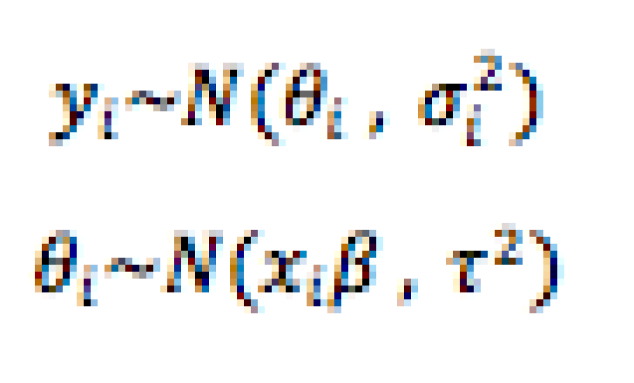
Where is the estimated effect size for the study population i, which has a normal distribution with mean representing the true effect size for such population, and is the within-study (i.e. sampling error) variance. In turn, is assumed to be a population-specific realization of the distribution of true effects for all effects, where its mean is parameterized as a function of some study-level variable(s) , and is the between-study (i.e. heterogeneity) variance. The combined two-level distribution is presented below [5]:

A linear regression model can be specified under this distributional assumption as follows [5]:

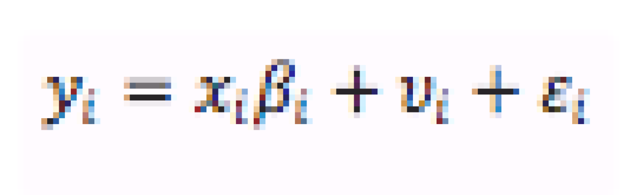
Where

is a random effect describing the study-specific deviation from the distribution mean, and

is a random error term describing sampling variability.

The assumption of a linear model and a specific distribution for the random effects makes this approach more suitable for continuous variable outcomes as opposed to measures based on count data or ratios. However, this model can be adapted to the latter situation by using log-transformed relative measures of association (log odds ratio, log risk ratio). However, this will impose a normal distribution to the random terms, with constant variance along the range of the outcome, when such error term is actually dependent on the value of the outcome.

4. Relationship to other statistical methods:

As can be appreciated from the model above, meta-regression can be regarded as a specific case of multilevel or mixed models. Other forms of integrative analytical techniques can also be fit into this framework. In this sense, random-effects meta-regression would be the most flexible of the integrative analytical techniques, because it allows simultaneously to estimate a random effect for differences between groups and allows to parameterize the expected value of the parameter of interest as a function of group-level variables (a fixed effect for differences between groups) θi=xiβ   . As opposed to this, random-effects meta-analysis estimates a random effect between groups, but it summarizes the expected value for the parameter of interest as the study-specific value θi , thus, a larger proportion of the between study variance is forced into the random parameter (i.e. larger standard errors). Finally, fixed effects meta-analysis is the more restricted version of this family of models, since it doesn’t use random or fixed effects to explain variability across studies, only the within study error term εi. We already mentioned that a fixed effects meta-regression is rarely an appropriate model, but it would be equivalent to a scenario where all the variability between studies is assumed to be explained by the fixed parameter xiβ, and no room is left for additional random variation between groups. The following graph helps to illustrate the relationship between meta-analysis and multilevel models. Since typically researchers conducting meta-analysis and meta-regression don’t have individual-level data, this family of models can be regarded as an “incomplete” multilevel model. The within variance is originated at a level below individual studies, but it cannot be estimated from the available data. Therefore, it must be assumed to be known; this has gained this family of models the namesake of V-known models [6].

Graph 2. Meta-analysis and meta-regression as hierarchical models

For those readers more familiar with weighted least squares regression than with multilevel models, it may be useful to think of meta-regression as a special case of it, where the weights are again the inverse of the variance for each study, which is the sum of the between and within variance components. There is an important difference, though because weighted least squares do not explicitly differentiate between the sources of variance, so it cannot properly take into account that part of the model variance is assumed to be known (within), while other part is estimated (between). This may lead to inadequate standard errors.

Finally, meta-regression can also be regarded as a more sophisticated method to explore effect measure modification, where the moderators are study-level variables. This goal can also be achieved through stratified or sub-group analysis, with the caveat that these latter methods estimate heterogeneity independently for each stratum or sub-group, therefore precluding direct statistical contrasts between groups.

5. Assumptions:

Assumptions of random effects meta-regression are specific versions of the normality and homoscedasticity assumptions:

1. All studies share a common τ2, i.e., they come from the same super-population of studies [7].

2. The observed sampling variances σi2 are the “true” variances within each study [4].

3. The distributional assumptions about the random effects and error terms are correct.

In reference to the latter assumption, it is relevant to highlight again the issue that arises with the estimation of the error term in models whose outcome parameter is dependent on proportions (OR, RR). In addition to these three assumptions, all other regular assumptions required to make inferences from a linear regression model still apply (i.e. linearity, independence, no omitted predictors, correct functional transformation of the predictors, error-free measurement, exchangeability assumptions, etc.).

6. Estimation algorithm

Fitting a random-effects meta-regression model departs from obtaining an estimate of the between-studies variance τ2. From then on additional parameters can be estimated using traditional methods. A summary of the algorithm steps is presented next:

1. Obtain an estimate of τ2: Depending on the type of data available, there are several procedures to do this:

   1. DerSimonian-Laird / method of moments: The DerSimonian-Laird method can be implemented to obtain a pooled estimate of the between variance when count data for the cells of 2×2 tables for a series of studies are available. The method of moments is a generalization of it. It is used in meta-regression as an inherited method from meta-analysis.

   2. Maximum likelihood: This is a conventional method of estimation, but may be less robust to the hierarchical structure of the data used in this type of analysis, thus resulting in inadequate standard errors.

   3. REML: This is the preferred method to fit both multilevel models and meta-regression models because it is unbiased and efficient. It estimates parameters that maximize the likelihood of the error distribution while imposing restrictions to avoid over-fitting. This will allow to obtain a better balance between the fractions of the variability captured by the fixed part vs. the random part of the statistical model.

   4. Empirical Bayes: Often times, the adequacy of the between variance estimates is questioned because it depends on the assumption that the within variance is fixed at the study level. Empirical Bayesian models can be used to characterize plausible distributions of such errors and tackling problems that may arise due to this artificial assumption. Extensive documentation on Bayesian method for meta-regression can be found in [8]. However, some authors have characterized the difference in estimates from REML and empirical Bayes as negligible.

   5. Other methods: There are other, less frequently used, estimators of τ2. These include the Hedges, Sidik-Jonkman and Hunter-Schmidt estimators.

2. Estimate fixed parameters and confidence intervals: This is performed using conventional methods (Newton-Raphson algorithm or other iterative algorithms).

3. Adjust results using any necessary corrections:

   1. Knapp-Hartung variance estimator: It is based on a t distribution rather than a normal distribution. Simulations have shown that confidence intervals based on this variance estimator perform better than z-based confidence intervals.

   2. Permutation-based CI and test statistics: This is also an alternative calculation of the variance and confidence intervals that can help to address the issue of using asymptotical approaches to estimate the variance in settings with very limited amount of observations and repeated testing (multiple group-level moderators).

4. Calculate additional parameters, tests, predictions, produce graphs, etc.: results from previous steps can be used to estimate heterogeneity, linear predictions, BLUPs, and certain useful graphs like forest plots, funnel plots, Baujat plots, and linear prediction plots. Details on graphical representation of meta-regression can be found in [10].

7. Interpretation:

The beta coefficients, confidence intervals, p-values and standard errors resulting from meta-regression are interpreted in the same manner than traditional coefficients from multi-level models. In addition to these, a typical meta-regression analysis will produce a number of parameters describing the model heterogeneity:

• τ2: It is an estimate of the residual between variance (between variance not captured by the fixed part of the model) expressed in squared units of the effect estimate. It may be cumbersome to interpret directly (e.g. imagine the variance of a log odds ratio, expressed in units of ln(OR)2).

• τ: A measure of residual between dispersion expressed in the same units as the effect estimate. This one may be easier to interpret when the effect estimate is a continuous variable (e.g. standard deviation of the mean difference in glucose between studies).

• I2: Estimates how much of the unaccounted variability (residual heterogeneity + sampling error) is attributable to residual heterogeneity. It is expressed as a percentage.

• H2: It estimates the ratio of the unaccounted variability relative to the sampling variability. In other words, it provides an estimate of how much our uncertainty about the parameter of interest is inflated due to consideration of all sources of variance, as opposed to a model where only within variance contributes to the width of the confidence intervals. Can be thought of as a multiplicative factor.

• R2adj: It is the estimated % of heterogeneity accounted for by the addition of predictors into the model as compared to an “empty” model. In other words, it is the percentage of the heterogeneity explained by the group-level variables in the model.

• Q: It is a χ2-based test statistic contrasting observed differences between studies vs. the differences expected by chance. It is to be noted that Q is typically an underpowered statistic, and that the typical analytical scenario for meta-regression, where only a small number of observations is available may lead to both high rates of false discovery and failure to detect an existing association.

Graphical interpretation:

Funnel plots are equivalent to those used in meta-analysis. Forest plots instead may be slightly different, since they do not include an overall pooled estimate. Instead, they may include multiple study-level Bayesian credibility intervals centered on BLUPs. One peculiarity is that observed point estimates may lie outside the credible intervals due to Bayesian shrinkage. This occurs because the BLUP based intervals “pull” the observed values towards the linear prediction with a “force” inversely proportional to the credibility of the observed values (e.g., study No. 26 below).

Graph 3. Meta-regression forest plot example, using the cholesterol dataset published in[7]

The Baujat plot is a graph of the influence of individual studies on the beta coefficients vs. its relative contribution to the pooled heterogeneity estimate. Studies falling away from the mass of observations in a Baujat graph should be further investigated to understand and address the reasons of such simultaneously outstanding heterogeneity and influence (e.g. studies 30 and 49 below).

Graph 4. Example of a Baujat plot in meta-analysis or meta-regression

Meta-regression linear prediction plots often use bubbles instead of points to represent each analyzed data point. The bubbles are drawn with sizes proportional to the contribution of individual studies towards the linear prediction, i.e. proportional to the inverse variance.

Graph 5. Example of a bubble plot with linear predictions, using the using the cholesterol dataset published in [7]

In the graph above, the solid line represent linear predictions for the odds ratio as a function of the mean absolute reduction in cholesterol observed at the group level. Dot lines are 95% confidence bands. The bubbles are the observed log odds ratios for each study, with bubble sizes proportional to the study weights. The horizontal dashed line represents the null association scenario.

8. Common misunderstandings:

The design, implementation and interpretation of a meta-regression model is a complex process prone to errors and misunderstandings. Some of the most frequent ones are highlighted below:

9.  

    

   Theoretical and practical limitations:

In spite of the apparent fanciness of the meta-regression methods, there are numerous limitations that can impair the ability of the model to make valid inferences. In first place, sample size is often insufficient to perform a meta-regression. Some estimation methods are based on asymptotical assumptions and can easily be biased when the sample size is small. In addition, published papers may not always measure or appropriately report the information on covariates needed for the model. These two precedent points may result in the inability to properly adjust for confounding. Even if the information on confounders is present and the number of studies is moderately large, characteristics of the studies tend to be correlated, giving rise to problems of collinearity [9].

Moreover, meta-regression analysis will always be subject to the risk of ecological fallacy, since they attempt to make inferences about individuals using study-level information. Also, it is sometimes difficult to interpret the effect of aggregate variables without the ability to condition on the individual-level analogous measurements (e.g. median neighborhood income without information on individual income). It has also been noticed that non-differential measurement error at the individual level may be able to bias group-level effects away from the null.

Finally, literature reviews are always susceptible to publication bias, and in particular, quantitative methods are subject to the risk of data dredging and false positive findings.

10. Applications:

In first place, it is important to realize that meta-regression is not always necessary. Sometimes, a meta-analysis may be sufficient to summarize the published information. Meta regression may be more useful when there is substantial heterogeneity (even if not statistically significant). A rough guide for the interpretation of the amount of heterogeneity is shown below [1]:

• I2 from 0% to 40%: might not be important

• I2 from 30% to 60%: may represent moderate heterogeneity

• I2 from 50% to 90%: may represent substantial heterogeneity

• I2 from 75% to 100%: considerable heterogeneity

Meta-regression should be planned and incorporated in the literature review protocol when it is interesting to explore study-level sources of heterogeneity, especially if there are variables suspected or known to modify the effect of the explored risk factors.

Meta-regression may be useful when there is a wide range of values in a continuous moderator variable, but relatively few studies with the exact same value for that moderator. By contrast, meta-regression may not be feasible when there is too little variability in the observed values of the moderators of interest.

Meta-regression serves to appropriately combine and contrast multiple subsets of studies (e.g. by study design, or by individual measurement procedures) when a single summary measure does not seem correct or sufficient to capture all the clinical or methodological diversity in those subsets.

Meta-regression can also serve to implement network meta-analysis. In this case, the model will use information about a parameter calculated in individual study groups defined by levels of exposure(s). For instance, instead of using the study specific log OR as an outcome, it is possible to model the log odds in each contrasted group (placebo, exposure1, exposure2, etc.). Then, the exposure specification can be used in meta-regression as a moderator of the log odds to obtain a log OR.

11. Summary and conclusions

Meta-regression is a powerful tool for exploratory analyses of heterogeneity and for hypothesis generation about cross-level interactions. Occasionally, it may help to test hypothesis of such effect measure modifications as well as to inform health decision making, as long as the interaction hypothesis are stated a priori and substantiated in scientific theory.

Meta-regression may also help to better understand the sources of variability in meta-analysis and to adequately summarize published information in a richer manner than a single number or point estimate does. Furthermore, it is easy to relate meta-regression to the increasingly popular multilevel modeling methods. The popularity of the latter may help to make meta-regression results easier to interpret and communicate.

However, it needs to be performed with extreme caution, because it is prone to error, poor methodological implementation, and misinterpretations.

Readings

[1]  Higgins J, Green S (editors). 9.5 Heterogeneity, and 9.6. Investigating heterogeneity. In Cochrane Handbook. Syst. Rev. Interv. Version 5.1.0 [updated March 2011]. Cochrane Collab. 2011.

Provides a clear definition of statistical heterogeneity and its sources in lay terms. Gives a guideline to quantitatively interpret I^2 coefficient. Gives an interpretation of the confidence intervals for the pooled estimates from random effects vs. fixed effects meta-analysis. Gives a very brief conceptual summary of what meta-regression is, why random effects meta-regression is preferred, why the number of available studies and the number of moderators is relevant, and why study-level moderators should be specified a priori.

[2]  Petitti D. Meta-Analysis, Decision Analysis, and Cost-Effectiveness Analysis: Methods for Quantitative Synthesis in Medicine. 1994.

This book provides an extraordinarily clear and intuitive definition and interpretation of statistical heterogeneity, variance components and sources of variability in meta-analysis and the differences and paradoxes of random effects vs. fixed effects analytical techniques. It is a great starting point to initiate an exploration of the topic.

[3]  Borenstein M, Hedges L V, Higgins JPT, Rothstein HR. Chapter 20. Meta-Regression. Introd. to Meta-Analysis, 2009, p. 187–204.

Provides a definition of meta-regression highlighting its analogy with single level regression. It includes a worked example on meta-regression for a BCG vaccine. Presents some useful graphs such as the bubble plot. Clearly states the differences in the hypothesis being tested in random effects vs. fixed effects models. Describes an interpretation for T^2. It is focused on the random effects meta-regression, describing the procedures for the calculation and interpretation of heterogeneity test statistics, R^2 and T^2.

[4]  Hartung J, Knapp G, Sinha B. Chapter 10. Meta-Regression. Stat. Meta-Analysis with Appl., 2008, p. 127–37.

It states that meta-regression is more useful on the presence of substantial heterogeneity. Provides statistical models for meta-regression in a language that is akin to multilevel models. Provides to estimate the parameters theta, beta, and variance-covariance matrices in random effects meta-regression. It also provides formulas to derive confidence intervals for those parameters. Contrasts the MM and REML versions of the variances estimators. Describes three cases with an “empty” model (meta-analysis), model with 1 covariate (simple meta regression), and more than 1 covariate (multivariable meta-regression). It states the statistical model in matrix notation. Describes some applications of metaregression: explaining heterogeneity, appropriately combining subsets of studies, combining controlled and uncontrolled trials.

[5]  Chen D-G (Din), Peace KE. Chapter 7. Meta-Regression. Appl. Meta-Analysis with R, 2013, p. 177–212.

Describes meta-regression as an extension of regular weighted multiple regression, describes fixed effects MR as more powerful, but less reliable if between-study variation is significant. Describes statistical model for level 2 variables. Explicitly states analogy with mixed models. Presents extended examples using R. Lists several methods available to estimate between variance. Compares meta-regression vs. weighted regression and highlights differences in the assumed error distribution.

[6]  Dias S, Sutton AJ, Welton NJ, Ades A. NICE DSU technical support document 3: heterogeneity: subgroups, metaregression, bias and bias-adjustment.

Compares advantages and disadvantages of different options to explore heterogeneity. Provides a slightly different statistical parameterization of the model using a Bayesian perspective on Meta-Regression. Provides code for analysis implementation in WinBUGS. Presents applications to network meta-analysis and regression on baseline risk. Clearly states assumption of equal effect of moderator across groups. Highlights the importance of centering predictors. Discusses appropriateness of tests and information criteria in Bayesian context. Describes the appropriateness of one and two-step approaches to individual patient data meta-analysis.

[7]  Harbord R, Higgins J. Meta-regression in Stata. Stata J 2008;8:493–519.

Presents statistical model relating it to multilevel models and presents a conditional notation for the different types of integrative methods (fixed effects and random effects meta-analysis, meta-regression). It describes in detail how to implement these models in Stata, including statistical and graphical representations. A very valuable practical resource.

[8]  Viechtbauer W. R documentation for the package “metafor.” 2015.

Presents the statistical model, different types of estimation methods, heterogeneity parameters and their interpretation for univariate and multivariate regression models. It describes in detail how to implement these models in R, including statistical and graphical representations. A very valuable practical resource.

[9]  Thompson SG, Higgins JPT. How should meta-regression analyses be undertaken and interpreted? Stat Med 2002;21:1559–73.

Describes in great detail the interpretation, limitations, pitfalls and common misunderstandings of the meta-regression model. It is an extraordinarily valuable resource to develop a critical mindset about the method.

[10]  Thompson SG, Sharp SJ. Explaining heterogeneity in meta-analysis: a comparison of methods. Stat Med 1999;18:2693–708.

Describes different approaches to explore heterogeneity using association parameters as outcome or log proportions or logits as group-level outcomes. Describes appropriateness of the REML estimation method.

[11]  Anzures-Cabrera J, Higgins JPT. Graphical displays for meta-analysis: An overview with suggestions for practice. Res Synth Methods 2010;1:66–80.

Describes and prescribes some recommendations for graphical representation of integrative methods.

Additional resources (more detailed statistical methods, discipline-specific applications, and topics which are covered in more detail elsewhere):

[12]  Stanley TD, Jarrell SB. Meta-Regression Analysis: A Quantitative Method of Literature Surveys. J Econ Surv 1989;3:161–70.

[13]  Berkey C, Hoaglin D, Mosteller F, Colditz G. A random-effects regression model for meta-analysis. Stat … 1995;14:395–411.

[14]  Van Houwelingen HC, Arends LR, Stijnen T. Advanced methods in meta-analysis: multivariate approach and meta-regression. Stat Med 2002;21:589–624.

[15]  Abrams K, Sanso B. APPROXIMATE BAYESIAN INFERENCE FOR RANDOM EFFECTS META-ANALYSIS. Stat Med 1998;17:201–18.

[16]  Stanley T. Wheat From Chaff: Meta-Analysis As Quantitative Literature Review. J Econ Perspect 2001;15:131–50.

[17]  Bellavance F, Dionne G, Lebeau M. The value of a statistical life: a meta-analysis with a mixed effects regression model. J Health Econ 2009;28:444–64.

[18]  Stanley TD. Meta-Regression Methods for Detecting and Estimating Empirical Effects in the Presence of Publication Selection. Oxf Bull Econ Stat 2007;1:070921170652004 – ???

[19]   Jackson D, White IR, Riley RD. A matrix-based method of moments for fitting the multivariate random effects model for meta-analysis and meta-regression. Biom J 2013;55:231–45.

[20]  Higgins JPT, Thompson SG. Controlling the risk of spurious findings from meta-regression. Stat Med 2004;23:1663–82.

[21]  Viechtbauer W. Conducting Meta-Analyses in R with the metafor Package. J Stat Softw 2010;36:1–48.

[22]  Snijders T, Bosker R. 3. Statistical treatment of clustered data. Multilevel Anal. An Introd. to Basic Adv. Multilevel Model., n.d., p. 36–8.

[23]  Greenland S, O’Rourke K. Meta-Analysis. In: Rothman KJ, Lash TL, Greenland S, editors. Mod. Epidemiol., 2008, p. 673–7.