Kriging Interpolation
Overview
Kriging is a method of spatial interpolation that originated in the field of mining geology as is named after South African mining engineer Danie Krige.
Description
Kriging is one of several methods that use a limited set of sampled data points to estimate the value of a variable over a continuous spatial field. An example of a value that varies across a random spatial field might be average monthly ozone concentrations over a city, or the availability of healthy foods across neighborhoods. It differs from simpler methods, such as Inverse Distance Weighted Interpolation, Linear Regression, or Gaussian decays in that it uses the spatial correlation between sampled points to interpolate the values in the spatial field: the interpolation is based on the spatial arrangement of the empirical observations, rather than on a presumed model of spatial distribution. Kriging also generates estimates of the uncertainty surrounding each interpolated value.
In a general sense, the kriging weights are calculated such that points nearby to the location of interest are given more weight than those farther away. Clustering of points is also taken into account, so that clusters of points are weighted less heavily (in effect, they contain less information than single points). This helps to reduce bias in the predictions.
The kriging predictor is an “optimal linear predictor” and an exact interpolator, meaning that each interpolated value is calculated to minimize the prediction error for that point. The value that is generated from the kriging process for any actually sampled location will be equal to the observed value at this point, and all the interpolated values will be the Best Linear Unbiased Predictors (BLUPs).
Kriging will in general not be more effective than simpler methods of interpolation if there is little spatial autocorrelation among the sampled data points (that is, if the values do not co-vary in space). If there is at least moderate spatial autocorrelation, however, kriging can be a helpful method to preserve spatial variability that would be lost using a simpler method (for an example, see Auchincloss 2007, below).
Kriging can be understood as a two-step process: first, the spatial covariance structure of the sampled points is determined by fitting a variogram; and second, weights derived from this covariance structure are used to interpolate values for unsampled points or blocks across the spatial field.
The variogram
A variogram (sometimes called a “semivariogram”) is a visual depiction of the covariance exhibited between each pair of points in the sampled data. For each pair of points in the sampled data, the gamma-value or “semi-variance” (a measure of the half mean-squared difference between their values) is plotted against the distance, or “lag”, between them. The “experimental” variogram is the plot of observed values, while the “theoretical” or “model” variogram is the distributional model that best fits the data. Variogram models are drawn from a limited number of “authorized” functions, including linear, spherical, exponential, and power models (see examples below).

(Poilou 2008)
The choice of a variogram model is fundamentally user-defined, although statistical software can often help define best-fitting models using various approaches that include least-squares, maximum likelihood, and Bayesian methods. In the example below of variograms for cholera and dysentery rates in an area of Bangladesh, an exponential model has been chosen as the “best-fit” model for a variogram of cholera rates, while a spherical model fits the dysentery rates better. In both cases, the rising curve at short distances implies that locations that are closer together are more similar to each other than locations that are father apart. At a certain point (~300 meters for cholera and ~1000 meters for dysentery), the gamma values reach a plateau, indicating that the difference between rates at locations separated by this distance have reached the value of the overall sample variance.
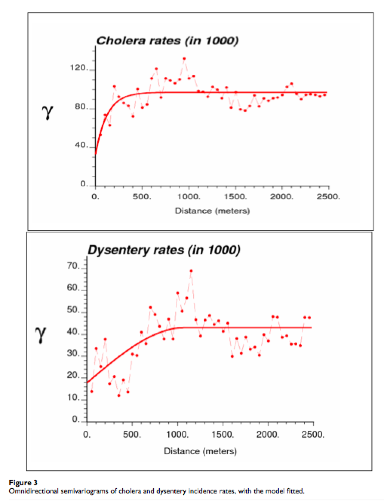
(Ali 2006)
The Kriging weights
Weights for each interpolated point are calculated according to the spatial structure of the interpolated location in reference to all the sampled points. The weights are determined from the variogram based on the spatial structure of the data, and are applied to the sampled points according to the formula:
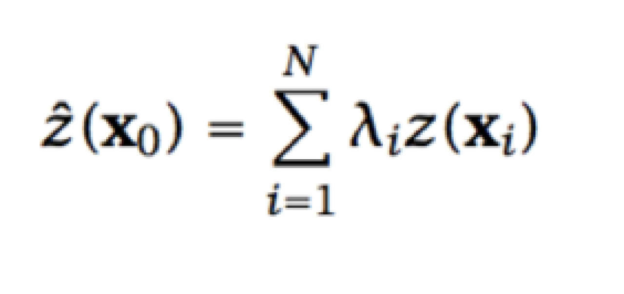
where the value of the predicted point (z-hat, at location x-nought) is equal to the sum of the value of each sampled point (x, at location i) times that point’s unique weight (lambda, for location i).
The covariance matrix from the estimated variogram is used to calculate the weights (slightly differently according to which type of kriging is being conducted).
Kriging assumptions
The two main assumptions for kriging to provide best linear unbiased prediction are those of stationarity and isotropy, though there are various forms and methods of kriging that allow the strictest form of each of these assumptions to be relaxed.
-
Stationarity – the joint probability distribution does not vary across the study space. Therefore, parameters (such as the overall mean of the values, and the range and sill of the variogram) do not vary across the study space. The same variogram model is assumed to be valid across the study space. A useful article that helps in understanding this concept is Stephen Henley’s The importance of being stationary.
-
Isotropy – uniformity in all directions
Types of kriging
There are several sub-types of kriging, including:
-
Ordinary kriging, for which the assumption of stationarity (that the mean and variance of the values is constant across the spatial field) must be assumed. This is one of the simplest forms of kriging, but the stationarity assumption is not often met in applications relevant to environmental health, such as air pollution distributions.
-
Universal kriging, which relaxes the assumption of stationarity by allowing the mean of the values to differ in a deterministic way in different locations (e.g. through some kind of spatial trend), while only the variance is held constant across the entire field. This second-order stationarity (sometimes called “weak stationarity”) is often a pertinent assumption with environmental exposures.
-
Block kriging, which estimates averaged values over gridded “blocks” rather than single points. These blocks often have smaller prediction errors than are seen for individual points.
-
Cokriging, in which additional observed variables (which are often correlated with each other and the variable of interest) are used to enhance the precision of the interpolation of the variable of interest at each location.
-
Poisson kriging, for incidence counts and disease rates
-
And more…
Limitations
-
Since the weights of the kriging interpolator depend on the modeled variogram, kriging is quite sensitive to mis-specification of the variogram model.
-
Similarly, the assumptions of the kriging model (e.g. that of second-order stationarity) may be difficult to meet in the context of many environmental exposures. Some newer methods (e.g. Bayesian approaches) have thus been developed to try and surmount these obstacles.
-
In general, the accuracy of interpolation by kriging will be limited if the number of sampled observations is small, the data is limited in spatial scope, or the data are in fact not amply spatially correlated. In these cases, a sample variogram is hard to generate, and methods such as land-use regression may prove preferable to kriging for spatial prediction.
Readings
Textbooks & Chapters
-
Nhu D. Le, James V. Zidek (2006). Statistical analysis of environmental space-time processes. New York: Springer, c2006.(Several chapters are useful but particularly Ch. 7, “Spatial Prediction: Classical Approaches”.)
-
Bivand, R. S., Pebesma, E. J., & Gómez-Rubio, V. (2008). Applied Spatial Data Analysis with R (2008th ed.). Springer. Ch. 8 “Interpolation and Geostatistics.”
-
Waller, Lance A ., and Carol A. Gotway. Applied spatial statistics for public health data. Vol. 368. John Wiley & Sons, 2004. Available here. (This textbook is an excellent resource that describes the application of spatial statistical methods to public health data. It serves as an introduction to epidemiologic research and GIS. All chapters are very useful and several topics were covered. For example, fundamental principals of epidemiologic research are described as well as management, mapping and reporting of spatial data. However, Chapter 8 discusses spatial interpolation in general and section 8.3, focuses on kriging and describes a few of the kriging methods.)
Methodological Articles
-
Rogers, D. J. & Sedda, L. Statistical models for spatially explicit biological data. Parasitology 139, 1852–1869 (2012). (Although intended for biologists interested in modeling species distributions, this article provides a comprehensive and understandable introduction to kriging and its applications in the biological sciences).
-
Matheron, G. Principles of geostatistics. Economic Geology 58, 1246–1266 (1963).(Matheron’s original formalization of kriging).
-
Henley, Stephen.The importance of being stationary.Earth Science Computer Applications, v.16, no.12, p.1-3 (2001). (Useful discussion of the concept of stationarity in geostatistics).
-
Zimmerman, D., Pavlik, C., Ruggles, A., & Armstrong, M. P. (1999). An experimental comparison of ordinary and universal kriging and inverse distance weighting.Mathematical Geology, 31(4), 375-390. (This article compares different interpolation methods (ordinary kriging, universal kriging, and inverse squared-distance weighting) using simulated data. The effects of the interpolation methods were tested for statistical significance).
Application Articles
-
Carrat, F., & Valleron, A. J. (1992). Epidemiologic mapping using the “kriging” method: application to an influenza-like epidemic in France. American journal of epidemiology,135(11), 1293-1300.(This article serves as an introduction to kriging in the context of epidemiology. It presents its advantages and describes steps of implementation of “ordinary kriging” as an example. The authors illustrated the technique through an application to data from 6 successive weeks of the influenza-like epidemic in France (1989-1990))
-
Auchincloss, A. H., Diez Roux, A. V., Brown, D. G., Raghunathan, T. E. & Erdmann, C. A. Filling the gaps: spatial interpolation of residential survey data in the estimation of neighborhood characteristics. Epidemiology18, 469–478 (2007). (This study uses a variety of spatial interpolation methods, including kriging, to estimate the availability of healthy foods across neighborhoods using a limited set of sampled data).
-
Jerrett, M. et al. Spatial analysis of air pollution and mortality in Los Angeles. Epidemiology 16, 727–736 (2005). (This study uses universal kriging along with a multiquadric interpolator to generate a smoothed air pollution surface for Los Angeles, which is then related to mortality from a variety of causes).
-
Ali, M., Goovaerts, P., Nazia, N., Haq, M.Z., Yunus, M., Emch, M. Application of Poisson kriging to the mapping of cholera and dysentery incidence in an endemic area of Bangladesh. Int J Health Geogr 5:45 (2006). (Aside from exposure estimation, another common application of kriging in the health sciences is in modeling disease incidence. Here Poisson kriging is used to map cholera and dysentery in Bangladesh).
-
Goovaerts,P., & Gebreab, S. (2008). How does Poisson kriging compare to the popular BYM model for mapping disease risks?. International journal of health geographics, 7(1), 6. (The article compares Bayesian spatial models with Poisson kriging first using lung and cervix cancer mortality rates from 118 counties and then using simulated data.)
-
Pouliou, T., Kanaroglou, P. S., Elliott, S. J. & Pengelly, L. D. Assessing the health impacts of air pollution: a re-analysis of the Hamilton children’s cohort data using a spatial analytic approach. Int J Environ Health Res 18, 17–35 (2008). (Sometimes, kriging may be not the most effective method to estimate relevant exposures. In this instance, land use regression fared better than universal kriging in capturing local variation in air pollution).
-
Mercer, L. D. et al.Comparing universal kriging and land-use regression for predicting concentrations of gaseous oxides of nitrogen (NOx) for the Multi-Ethnic Study of Atherosclerosis and Air Pollution (MESA Air). Atmos Environ 45, 4412–4420 (2011). (On the other hand, this study found universal kriging to perform as well or better than land-use regression models in predicting levels of nitrous oxide gases (NOx)in the Los Angeles area for the Multi-Ethnic Study of Artherosclerosis and Air Pollution (MESA) study).
-
Zhang, K. et al. Geostatistical exploration of spatial variation of summertime temperatures in the Detroit metropolitan region. Environ. Res. 111, 1046–1053 (2011). (The authors compare various types of kriging and other methods in mapping summertime temperature across a city).
-
Oliver, M. A., Webster, R., Lajaunie, C., Muir, K. R., Parkes, S. E., Cameron, A. H., … & Mann, J. R. (1998). Binomial cokriging for estimating and mapping the risk of childhood cancer. Mathematical Medicine and Biology, 15(3), 279-297.(The article describes Binomial Cokriging; the authors analyzed the distribution of childhood cancer in England and estimated the risk of cancer using ordinary and conditional unbiased Cokriging. Their method of calculating risk geostatistically, took in to account correlated values of children living in nearby electoral wards)
Software
SAS
-
The KRIGE2D procedure
[removed]
R
Several packages are available in R to conduct interpolation by kriging, including “kriging” (simple package covering ordinary kriging), “gstat” (enables many forms of kriging including ordinary, universal, block, etc.), “geoR” and “geoRglm” (for Bayesian kriging). Below are some resources that pertain to the “kriging” and “gstat” packages.
- Documentation of package “kriging” – conduct and plot using ordinary kriging
[removed]
- Tutorial on kriging using package “gstat”
[removed]
Matlab/GNU Octave
-
mGstat – A Geostatistical Matlab toolbox
-
DACE – Design and Analysis of Computer Experiments. A matlab kriging toolbox
Websites
-
Geostatistics in Three Easy Lessons – Materials from Geoff Bohling’s course at Kansas University
-
ArcGIS Resources Center: How Kriging works – This is a great website providing a simple introduction to kriging
-
Project 5: Kriging Using The Geostatistical Analyst – Brief webpage describing the use ofGeostatistical Wizard to run ordinary kriging analyses.
Courses
Online Courses:
-
Practical Geostatistics 2000 – 2: Spatial Statistics (Self-paced online course from Edumine (main audience the mining industry))
-
Spatial Analysis Techniques in R taught by Professor David Unwin. The course is offered by Statictics.com and its main objective is to introduce R for geographic information analysis using R. it covers point pattern analysis, lattice objects and geostatistical data (including but not limited to kriging).
In-person Courses:
-
Applied Spatial Statistics at the Yale School of Forestry and Environmental Studies (Topics include spatial sampling, visualizing spatial data, quantifying spatial association and autocorrelation, interpolation methods, fittingvariograms, kriging, and related modeling techniques for spatially correlated data.)
-
An EPIC course is offered briefly introducing spatial epidemiology